Detecting Model Degeneration with a Probe

Authors: Lorenzo Baggi, Marco De Negri, Luca Sartori, Moritz Reihs (ETH Zurich)

Category: Interpretability / probing — an exploratory finding paired with a live demo. We train a lightweight linear probe on the internal activations of `Apertus-8B-Instruct-2509` and show that the onset of repetitive "degeneration" is linearly readable from a single hidden layer, early enough to enable real-time detection.

1. TL;DR

Language models sometimes collapse into repetitive, low-information loops. We show this failure is already visible inside the model before it surfaces in the text: a small linear probe (a lightweight classifier read off a frozen model's hidden states), trained with LoRA on Apertus-8B-Instruct-2509, recovers a per-token repetition score from a single layer — and degenerating tokens occupy a visibly distinct region of the hidden space. Try it live: interactive demo.

2. What is model degeneration?

Model degeneration is a failure mode of autoregressive language models in which generation collapses into repetitive, low-information output. The model gets trapped in a loop, producing the same phrase, sentence, or reasoning pattern over and over, while the text loses all semantic value. It does not stop generating; it simply stops communicating.

To see why this happens, recall how these models work. Autoregressive models generate text one token at a time: at each step the model looks at all previous tokens and picks the next one according to a probability distribution. When that distribution becomes too concentrated on a narrow set of tokens, often ones that are already present in the context, the model enters a self-reinforcing cycle it cannot escape on its own. This is the "curious case of neural text degeneration" first characterised by Holtzman et al. (arXiv:1904.09751), and it connects to the more recent open question of why reasoning models loop in the first place (Pipis et al., arXiv:2512.12895).

Across the completions we collected, degeneration takes several recurring forms. The repeated unit may be a single token, a digit or a word emitted hundreds of times, a short phrase, a full sentence reproduced verbatim, a mathematical expression, or a structural marker such as a row of asterisks or hashtags. In each case the model stops advancing the task and instead recycles material already present in its own output.

Importantly, the effect is strongly correlated with prompt difficulty: simple questions are answered cleanly, whereas hard, multi-step reasoning — competition mathematics above all — degenerates far more often. Once a loop sets in, the model frequently (though not always) fails to recover a natural stopping signal and keeps emitting tokens at full confidence until the generation is cut off by the token limit. The example below shows exactly this behaviour in Apertus-8B-Instruct-2509.

3. A concrete example

Consider a one-line arithmetic question drawn from our balanced dataset, run through Apertus-8B-Instruct-2509:

Prompt: What is the largest prime factor of 3328?

The model factorises the number correctly and even spots that 13 is prime — the answer is right there — but as it starts to list the factors it falls into a loop, repeating the digit "2" thousands of times and never delivering the answer:

To find the largest prime factor of 3328, we first need to find the prime factors of 3328. We can do this by dividing 3328 by the smallest prime number, which is 2.

3328 ÷ 2 = 1664 → 1664 ÷ 2 = 832 → … → 26 ÷ 2 = 13

Since 13 is a prime number, we have found all the prime factors of 3328.

The prime factors of 3328 are 2, 2, 2, 2, 2, 2, 2, 2, 2, 2, 2, 2, … [the digit "2" repeats until the generation hits its length limit; the correct answer, 13, is never given].

So what? The model is not confused about the mathematics — it solved the problem — yet the output is useless. This is the gap our work targets: the failure is in the generation dynamics, not the knowledge, which is exactly the kind of failure an internal probe might catch.

4. Dataset

Our starting point is the token-level dataset published on Hugging Face by Luca Sartori: `luca-sartori/degeneration-probe-instruct-token-level`. It contains 83,350 completions generated by Apertus-8B-Instruct-2509 across five public instruction datasets — one response per prompt — each annotated at the token level with a continuous repetition score.

The five source datasets span a deliberate range of difficulty, which matters because difficulty drives degeneration (Figure 1):

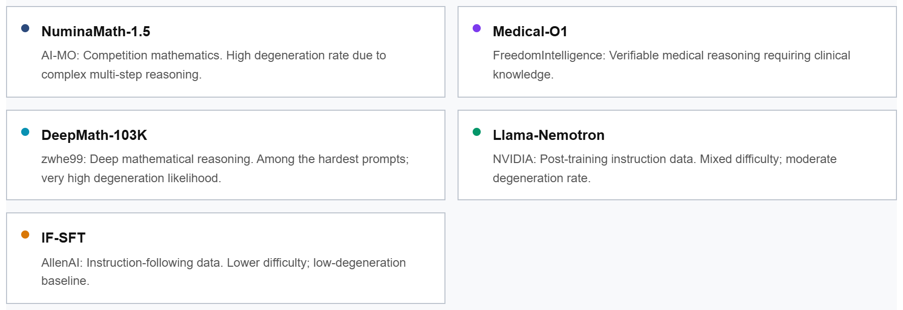
Figure 1 — The five public instruction datasets used as sources. NuminaMath-1.5 (AI-MO) and DeepMath-103K (zwhe99) are competition / deep mathematics and degenerate the most; Medical-O1 (FreedomIntelligence) is verifiable clinical reasoning; Llama-Nemotron (NVIDIA) is mixed-difficulty post-training data; and IF-SFT (AllenAI) is easier instruction-following data that serves as a low-degeneration baseline.

The class-imbalance problem. A generation is labelled positive (degenerating) if it contains at least one token whose averaged repetition score is ≥ 0.8; otherwise it is labelled negative (clean). In the full 83k corpus, the vast majority of completions are clean: the natural positive-to-negative ratio is roughly 1 : 72 (1.4% positive vs. 98.6% negative). Training a probe on such an imbalanced set would bias it toward always predicting "clean," so we downsampled the negative examples.

Concretely, we randomly removed negative examples using a fixed seed (42) for reproducibility. After a cleanup step that discarded rows with no scored tokens, the final corpus settled at 2,973 generations with a ratio of approximately 1 : 1.6 (38% positive vs. 62% negative); Figure 2 shows the class balance before and after this downsampling. The balanced dataset is published at `lorenzo0312/degeneration-probe-instruct-token-level-balanced`.

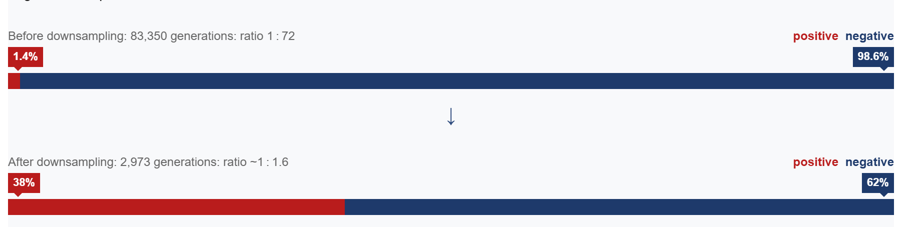
Figure 2 — Class balance before and after downsampling. Before (top): of 83,350 generations only 1.4% are positive (degenerating, red) against 98.6% negative (clean, blue), a 1 : 72 ratio. After downsampling the negative class (bottom): 2,973 generations at 38% positive vs. 62% negative, a ~1 : 1.6 ratio. So what? Downsampling turns a pathologically skewed corpus into one a probe can actually learn from, without discarding any of the rare positive examples.

The balanced corpus is split into train, validation, and test sets as follows (Figure 3):

Figure 3 — Train / validation / test split. The ~1 : 1.6 positive-to-negative ratio is preserved across all three splits (Train: 915 / 1,464; Validation: 113 / 186; Test: 113 / 182), so the probe is evaluated on the same class balance it was trained on.

By source, the math datasets dominate, which reflects where degeneration actually occurs (Figure 4):

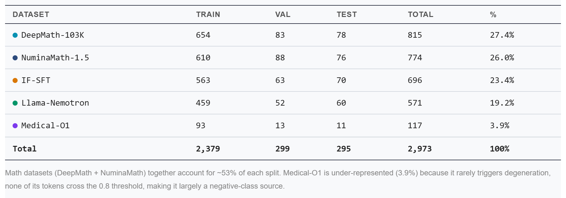
Figure 4 — Prompts per source dataset, across splits. DeepMath-103K (27.4%) and NuminaMath-1.5 (26.0%) together account for ~53% of each split, while Medical-O1 makes up only 3.9%. So what? Medical-O1 is under-represented because it rarely triggers degeneration — none of its tokens cross the 0.8 threshold — making it largely a negative-class source; the balanced set therefore concentrates supervision precisely where the failure mode lives.

5. How we labelled the data

Every completion in the corpus was generated by Apertus-8B-Instruct-2509, and every token receives a continuous repetition score between 0 and 1. A score of 0 means every bigram (every consecutive pair of tokens) in the surrounding context is unique — healthy, diverse output. A score of 1 means all bigrams repeat — a fully degenerate loop. A token is flagged as degenerating when its score is ≥ 0.8.

Our approach. Rather than looking at a single token in isolation, we look at the neighbourhood around it. We slide a window of 256 tokens along the generation and compute a bigram repetition score for each window position; a token then inherits the average score of all windows that contain it. This proceeds in two steps.

Step 1 — Bigram repetition score per window. For every 256-token window starting at position t we compute:

rep(t) = 1 − TTR(bigrams in tokens[t … t+255])

Here TTR (Type-Token Ratio) = unique bigrams ÷ total bigrams. Intuitively, if you keep seeing the same two-token pair over and over, the TTR is low and therefore rep(t) is high. A window where every consecutive pair of tokens is different gives TTR = 1 and rep(t) = 0.

Step 2 — Average across all windows containing the token. A token at position i belongs to every window starting between i−255 and i (up to 256 windows for tokens deep in a long generation). Its final score is the mean of all those window scores. This smoothing prevents a single high-repetition burst from unfairly tainting isolated tokens far from the loop. If the resulting score is ≥ 0.8, the token is flagged as degenerating. Figure 5 traces this computation for a single token.

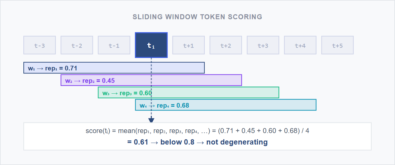
Figure 5 — Sliding-window token scoring. A schematic of how one token's score is computed. The highlighted token tᵢ sits inside four overlapping 256-token windows with bigram-repetition scores rep₁ = 0.71, rep₂ = 0.45, rep₃ = 0.60, rep₄ = 0.68. Its final score is the mean of all containing windows: (0.71 + 0.45 + 0.60 + 0.68) / 4 = 0.61 — below the 0.8 threshold, so this token is not flagged as degenerating.

One edge case is worth noting: tokens that fall outside any complete 256-token window (only possible in generations shorter than 256 tokens) receive a null repetition score and are excluded from training.

6. Training the probe

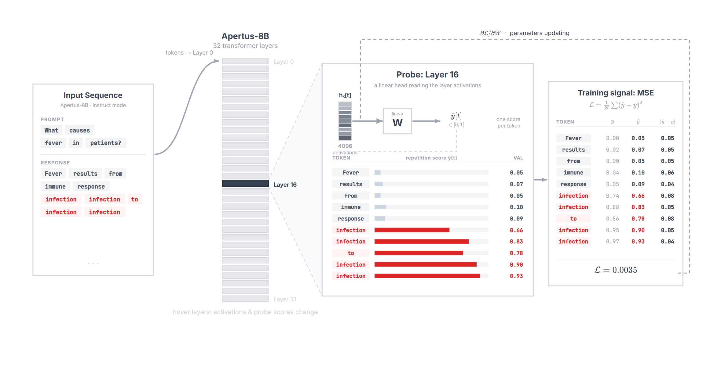
A probe is a lightweight linear head attached to one internal layer of the language model; it tests what information that layer's representations already contain. The technique of reading information off a frozen model's intermediate activations with a simple linear classifier was introduced by Alain & Bengio (arXiv:1610.01644). During a forward pass, the prompt and response are fed through Apertus-8B-Instruct-2509; at a chosen layer X the probe intercepts the hidden state hₜ for every token t and maps it to a scalar score in [0, 1] via a linear projection followed by a sigmoid.

Our approach. We keep the backbone frozen except for lightweight LoRA adapters. LoRA (Low-Rank Adaptation; Hu et al., arXiv:2106.09685) injects two small trainable matrices alongside each frozen attention weight matrix W — a down-projection A ∈ ℝ^(d×r) and an up-projection B ∈ ℝ^(r×d) — so the effective weight update is ΔW = BA with rank r ≪ d (typically r = 8–64). Only A and B are trained; W stays unchanged. This reduces the number of trainable parameters by several orders of magnitude while still letting the representations adapt to the probe task.

The training signal is the Mean Squared Error between the probe's predicted score ŷₜ and the pre-computed repetition label yₜ for each token:

ℒ = (1/N) · Σₜ (ŷₜ − yₜ)²

Tokens with a null repetition label are excluded. We chose a regression formulation rather than binary classification because it gives the probe a continuous gradient signal across the full score range, instead of a hard boundary at 0.8. Figure 6 shows the full probe-training pipeline.

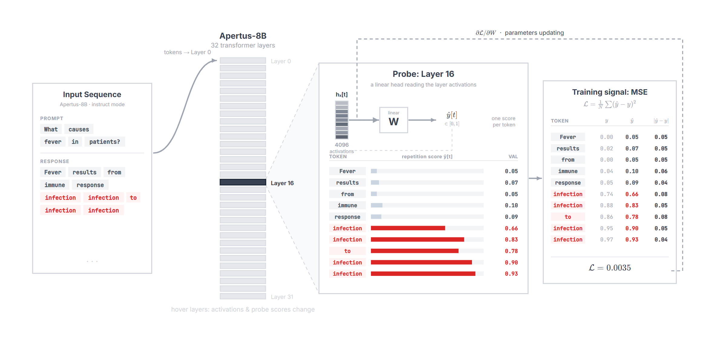
Figure 6 — Probe training pipeline. The probe attaches to a chosen layer (here layer 16), reads its 4,096-dimensional activations, and predicts a per-token repetition score ŷ[t] via a single linear weight W; the MSE loss against the deterministic target y[t] trains the probe (with the backbone frozen apart from LoRA adapters). On the right, per-token predictions are shown against their targets — degenerating tokens ("infection", "to") score near 0.9 while healthy tokens stay near 0.05. (An interactive version, where hovering a layer shows how activations and scores change with depth, is available in the live demo.)

Which layer is best? Each probe is trained independently on a single transformer layer. We swept across ten layers (10, 14, 18, 22, 24, 26, 28, 29, 30, 31) and found that layers from layer 20 onward all achieve similar detection performance, with only small differences in AUC across sources. Earlier layers are slightly weaker, and layer 31 (the very last) is the worst among the later ones. So what? This means the degeneration signal is broadly distributed across the second half of the network rather than localised in one special layer — so a practical detector can attach almost anywhere past the midpoint and still work well.

7. Visualising the internal representations

To understand what degenerating tokens have in common at the representation level, we saved the hidden states produced at each transformer layer for every generated token. It helps to first recall how Apertus-8B-Instruct-2509 is structured: it is a decoder-only transformer with 32 layers, each containing a multi-head self-attention mechanism (32 query heads, 8 key/value heads) followed by a feed-forward network, passing a residual stream of 4,096 dimensions from one layer to the next. At each token position, this 4,096-dimensional vector is the model's complete internal representation of everything it has processed so far (Figure 7).

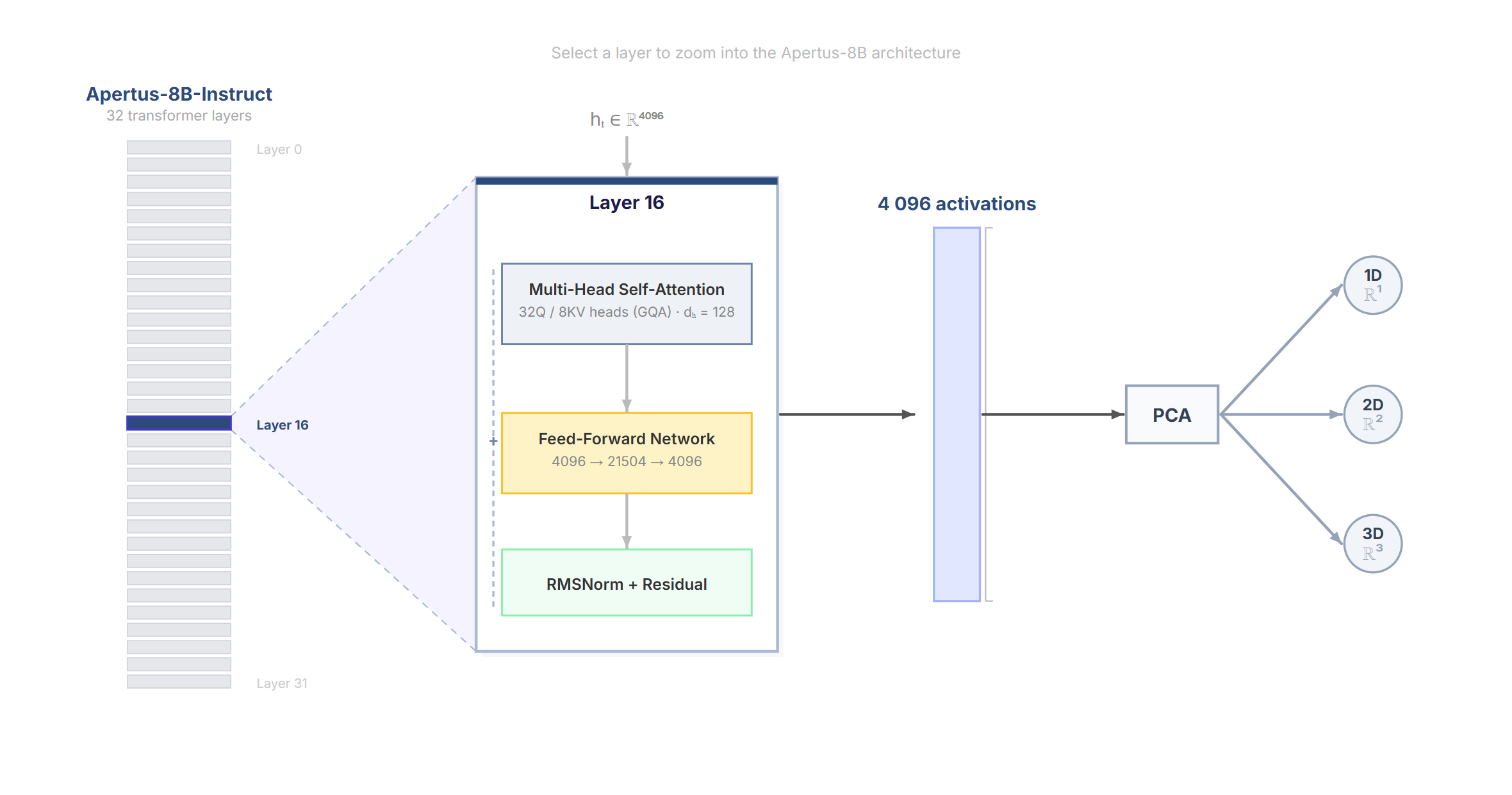
Figure 7 — Structure of one Apertus-8B transformer layer. Zooming into a single layer (here layer 16) of the 32-layer stack: a multi-head self-attention block (32 query / 8 key-value heads, grouped-query attention, head dimension 128), a feed-forward network (4096 → 21504 → 4096), and an RMSNorm + residual connection. The layer emits a 4,096-dimensional activation vector per token, which we then project with PCA to 1D / 2D / 3D. (Interactive version — hover any layer to zoom in — in the live demo.)

We extracted these hidden states at layers 1, 5, 10, 15, 20, 25, 30, and 31, for two model variants: the unmodified base model and the LoRA-finetuned one. We compared the two because we wanted the hidden states of degenerating and non-degenerating tokens to be more clearly separated, making the signal easier to isolate.

Our approach. To interpret what these 4,096-dimensional vectors encode, we applied PCA (Principal Component Analysis, a standard linear dimensionality-reduction technique that finds the directions of maximum variance) independently to each (layer, variant) pair, projecting the hidden states down to 1 and 2 dimensions. The logic is straightforward: if degenerating tokens occupy a geometrically distinct region of the hidden space, that structure should survive the projection and become visible. Because PCA is applied separately per (layer, variant) pair, each projection captures the directions of maximum variance within that specific set of representations, enabling a direct visual comparison between the base model and the LoRA-finetuned one. Each token is coloured by its repetition score, from green (healthy) to red (degenerating).

One caveat on reading these plots: the colour scale is normalised independently for each prompt, so it is not globally comparable across visualisations. A token with a score of 0.7 might appear green in one prompt and orange in another, depending on the range of scores within that prompt. The 0.8 flagging threshold, however, is fixed. Figure 8 shows the 2D projections for the base and LoRA models at layers 5, 10, and 30.

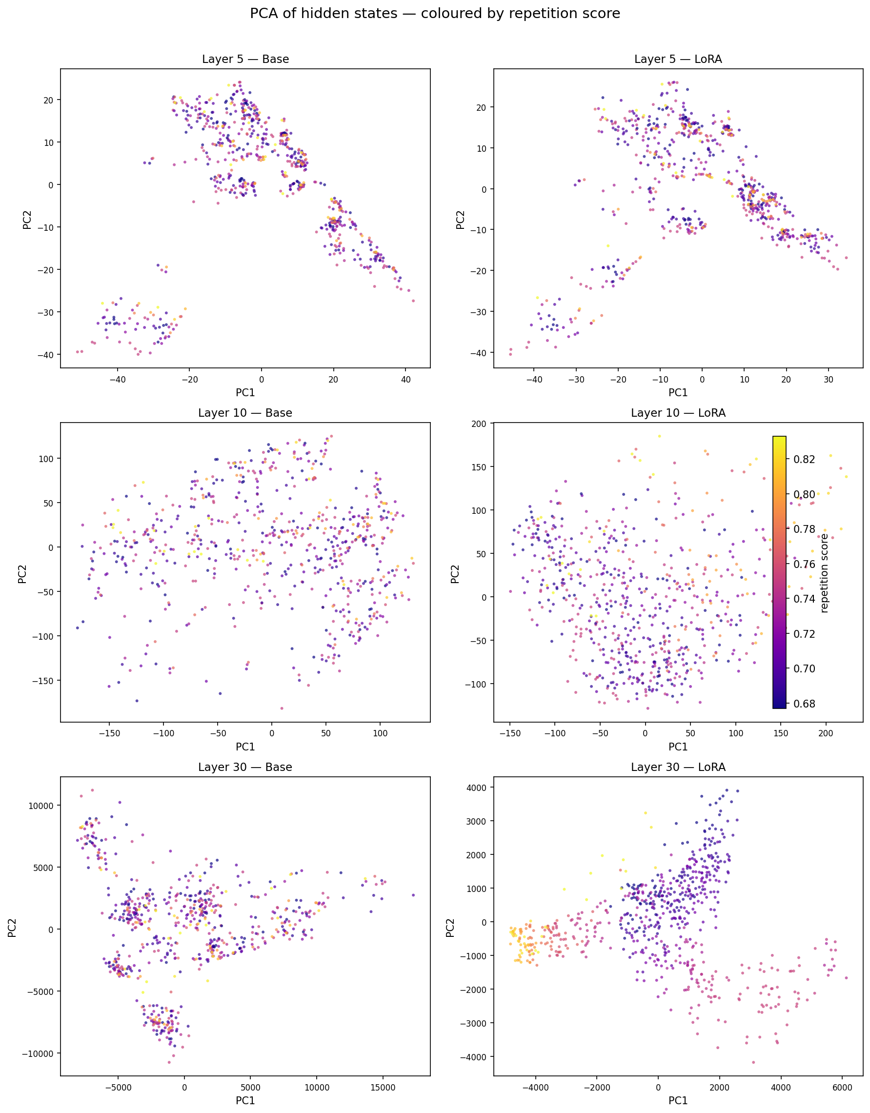
Figure 8 — 2D PCA of hidden states, base vs. LoRA, at layers 5 / 10 / 30. Each point is a token, coloured by repetition score (dark blue ≈ healthy, yellow ≈ degenerating). The left column is the base model, the right column is the LoRA-finetuned model. At layer 30 with LoRA (bottom right), the degenerating tokens form a compact cluster clearly separated from the healthy ones; LoRA consistently sharpens this separation across all layers. We also observed that LoRA increases the total variance explained by the first PCA components, particularly in the last layers, suggesting the finetuned model's representations are more structured and linearly separable. (An interactive, per-prompt version — where hovering a token highlights it across all six plots — is in the live demo.)

Figure 9 complements this with a parallel-coordinates view, tracing each token's 1D-PCA coordinate across layers.

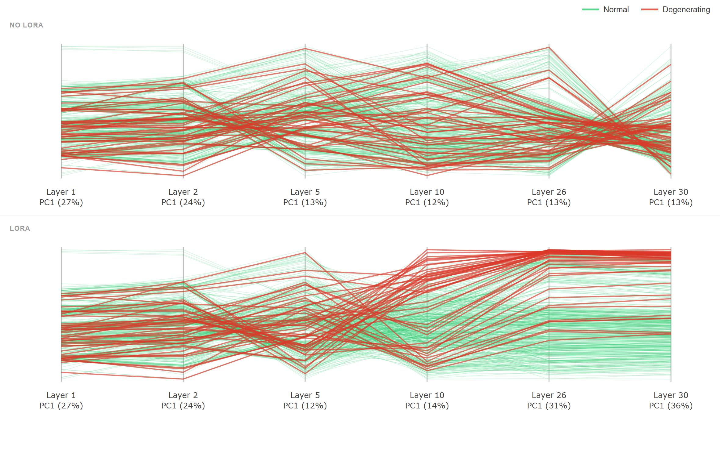
Figure 9 — Parallel-coordinates view: 1D PCA score across layers. Each line is a token, traced through its 1D-PCA coordinate at layers 1, 2, 5, 10, 26, and 30; green lines are healthy ("Normal") tokens and red lines are degenerating ones. The top panel is the base model ("NO LORA"), the bottom panel is the LoRA-finetuned model. As depth increases, the red trajectories diverge more sharply from the green ones, and the LoRA model (bottom) makes this divergence far more pronounced than the base model — confirming that fine-tuning concentrates the degeneration signal into a more linearly separable form. (Interactive version in the live demo.)

So what? The geometry corroborates the probe results from the other direction: degeneration is not just decodable by a trained classifier, it is visible as spatial structure in the raw representations — and LoRA fine-tuning makes that structure cleaner.

8. Conclusion

Lightweight linear probes, trained with LoRA-adapted hidden states from Apertus-8B-Instruct-2509, can recover the repetition score with good accuracy from a single internal layer. Layers from 20 onward are consistently the most informative, and the PCA projections show that degenerating and healthy tokens occupy visibly different regions of the hidden space well before the repetition becomes obvious in the generated text.

So what? This suggests that model degeneration is not only a surface-level symptom but is already encoded in the model's internal representations. A probe of this kind is cheap enough to run alongside generation, opening the door to real-time detection — and potentially to intervention: steering the model away from a loop as soon as the probe's score starts climbing, rather than only diagnosing the failure after the fact. This connects directly to the open question of why reasoning models loop in the first place (Pipis et al., arXiv:2512.12895).

Limitations. We want to be honest about the scope of the evidence. The balanced dataset used for training is relatively small (2,973 generations) and comes from a single model family, and the 0.8 threshold used to define "degenerating" is a useful but somewhat arbitrary cutoff. Extending this work to larger, multi-model datasets, and moving from passive detection to causal steering during generation, are natural next steps.

9. Try it & reproduce

• Live demo (interactive probe in your browser): parallelpanda.xaiml26.ivia.isginf.ch — runs base Qwen2.5-0.5B with a live degeneration probe, no setup. The full Apertus-8B-Instruct-2509 demo runs on the CSCS Clariden cluster.
• Balanced dataset: `lorenzo0312/degeneration-probe-instruct-token-level-balanced`
• Source dataset: `luca-sartori/degeneration-probe-instruct-token-level`
• Base model: `swiss-ai/Apertus-8B-Instruct-2509`

10. Acknowledgements

This project was carried out by Lorenzo Baggi, Marco De Negri, Luca Sartori, and Moritz Reihs at ETH Zurich, as part of the Explainable AI / Machine Learning (XAIML) course. We thank our supervisors Anna Hedström, Eduard Durech, and Valentina Pyatkin for their guidance throughout the project. We also thank the Swiss AI Initiative (ETH Zurich and EPFL) for the open Apertus model family that made this study possible, and CSCS for the Clariden compute access used for the Apertus-8B demo.

11. References

1. Swiss AI Initiative. Apertus: an open multilingual large language model from ETH Zurich and EPFL. 2024. `swiss-ai/Apertus-8B-Instruct-2509`
2. Holtzman, A., Buys, J., Du, L., Forbes, M., & Choi, Y. The Curious Case of Neural Text Degeneration. ICLR 2020. arXiv:1904.09751
3. Pipis, C., Garg, S., Kontonis, V., Shrivastava, V., Krishnamurthy, A., & Papailiopoulos, D. Wait, Wait, Wait… Why Do Reasoning Models Loop? arXiv, 2025. arXiv:2512.12895
4. Hu, E. J., Shen, Y., Wallis, P., Allen-Zhu, Z., Li, Y., Wang, S., Wang, L., & Chen, W. LoRA: Low-Rank Adaptation of Large Language Models. ICLR 2022. arXiv:2106.09685
5. Alain, G., & Bengio, Y. Understanding Intermediate Layers Using Linear Classifier Probes. ICLR Workshop 2017. arXiv:1610.01644